

KEEP GOING
[ml] 머신러닝 분류 classification 문제 뽀개기 본문
* 와인 종류를 분류하는 문제
https://heytech.tistory.com/149#
[Python] Random Forest 알고리즘 정의, 장단점, 최적화 방법
📚목차 1. 랜덤포레스트 정의 2. 랜덤포레스트 장단점 3. 실습코드 및 데이터셋 4. 코드 설명 1. Random Forest 정의 Random Forest는 의사결정나무 모델 여러 개를 훈련시켜서 그 결과를 종합해 예측하는
heytech.tistory.com
Tips
1. dir과 help 함수 이용하기
help(list.append)
help(pandas)
dir(pandas)
2. 어떤 모델을 선택할지 모르겠을 경우 랜덤포레스트 사용
from sklearn.ensemble import RandomForestClassifier
from sklearn.ensemble import RandomForestRegressor
3. 모듈이 설치되지 않았을 경우
pip install 모듈명
랜덤포레스트
오버피팅 문제를 해결하기 위해 앙상블 기법인 랜덤 포레스트를 적용한다.
앙상블 기법은 여러 개의 모델을 훈련하여 결과를 종합하여 예측하는 방법을 뜻한다.
train dataset에서 중복을 허용하여 샘플링한 데이터 셋으로 훈련하는 배깅 방식으로 각 의사결정나무 모델을 훈련한다.
라이브러리 import
import numpy as np
import pandas as pd
import warnings
warnings.filterwarnings(action='ignore') # 경고 메시지 무시
import matplotlib.pyplot as plt
import pickle # 객체 입출력
from sklearn.model_selection import train_test_split # 훈련/ 테스트 데이터 분리
from sklearn.preprocessing import StandardScaler # 정규화
from sklearn.ensemble import RandomForestClassifier as RFC # 랜덤포레스트 분류 알고리즘
from sklearn.tree import DecisionTreeClassifier as DTC # 의사결정나무 분류 알고리즘
from sklearn.ensemble import GradientBoostingClassifier as GBC # 그래디언트 부스팅 분류 알고리즘
# 모델 평가
from sklearn.metrics import accuracy_score, precision_score, recall_score, f1_score, confusion_matrix
데이터 불러오기
1. pd.read_csv
만약 구분자가 ';'인 경우 sep=';'
헤더가 없는 파일이라면 header=None
names=['a', 'b']를 통해 컬럼명 부여 가능
import pandas as pd

train = pd.read_csv('train.csv', sep=';')
test = pd.read_csv('test.csv', header=None)
submission = pd.read_csv('submission.csv', header=None, names=['a', 'b'])
2. x, y 데이터로 train, test 세트 구분하기(train, test 비율은 7:3으로 고정. random_state=42로 고정)
from sklearn.model_selection import train_test_split

x_train, x_test, y_train, y_test = train_test_split(x, y, test_size=0.3,random_state=42)
3. 데이터 확인
train.head(4)
데이터 전처리
1. 변수 제거
와인 분류(화이트/레드)에 영향을 주지 않는 변수 제거
불필요한 설명 변수(=독립변수)를 제거
# 와인 퀄리티가 와인 종류 구분에 영향을 주지 않음
red = red.drop(['quality'], axis=1)
white = white.drop(['quality'], axis=1)
2. 결측치 처리
해당 데이터프레임의 컬럼별 결측치 확인
red.isnull().sum()
white.isnull().sum()
3. 이상치 시각화
와인 종류에 따라 설명변수 데이터의 분포가 다를 수 있기 때문에 이상치는 설명변수별로 처리함
boxplot을 활용하여 모든 설명변수를 시각화
def boxplot_vis(data, target_name):
    plt.figure(figsize=(30, 30))
    for col_idx in range(len(data.columns)):
        # 6행 2열 서브플롯에 각 feature 박스플롯 시각화
        plt.subplot(6, 2, col_idx+1)
        # flierprops: 빨간색 다이아몬드 모양으로 아웃라이어 시각화
        plt.boxplot(data[data.columns[col_idx]], flierprops = dict(markerfacecolor = 'r', marker = 'D'))
        # 그래프 타이틀: feature name
        plt.title("Feature" + "(" + target_name + "):" + data.columns[col_idx], fontsize = 20)
    plt.savefig('../figure/boxplot_' + target_name + '.png')
    plt.show()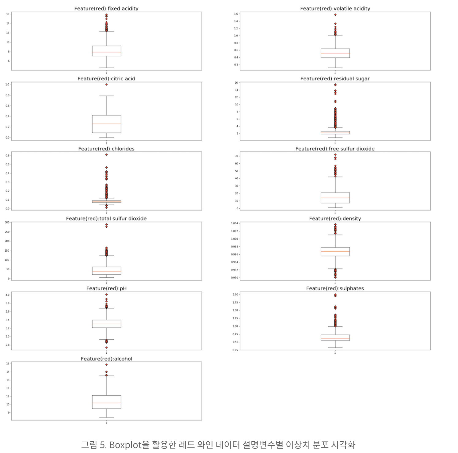
마찬가지로 화이트 와인에 대해서도 이상치 시각화 진행
만약 두 와인 종류를 결합한 후 이상치를 검증했다면 소중한 데이터가 이상치로 분류되어 활용되지 못했을 것임
따라서 분류 문제에서는 두 데이터를 분류해서 이상치 검증 필요
4. 이상치 제거
def remove_outlier(input_data):
    q1 = input_data.quantile(0.25) # 제 1사분위수
    q3 = input_data.quantile(0.75) # 제 3사분위수
    iqr = q3 - q1 # IQR(Interquartile range) 계산
    minimum = q1 - (iqr * 1.5) # IQR 최솟값
    maximum = q3 + (iqr * 1.5) # IQR 최댓값
    # IQR 범위 내에 있는 데이터만 산출(IQR 범위 밖의 데이터는 이상치)
    df_removed_outlier = input_data[(minimum < input_data) & (input_data < maximum)]
    return df_removed_outlier
# 이상치 제거한 데이터셋
red_prep = remove_outlier(red)
# 목표변수 할당
red_prep['target'] = 0
# 결측치(이상치 처리된 데이터) 확인
red_prep.isnull().sum()
# 이상치 포함 데이터(이상치 처리 후 NaN) 삭제
red_prep.dropna(axis = 0, how = 'any', inplace = True)
print(f"이상치 포함된 데이터 비율: {round((len(red) - len(red_prep))*100/len(red), 2)}%")# 이상치 제거한 데이터셋
white_prep = remove_outlier(white)
# 목표변수 할당
white_prep['target'] = 1
# 결측치(이상치 처리된 데이터) 확인
white_prep.isnull().sum()
# 이상치 포함 데이터(이상치 처리 후 NaN) 삭제
white_prep.dropna(axis = 0, how = 'any', inplace = True)
print(f"이상치 포함된 데이터 비율: {round((len(white) - len(white_prep))*100/len(red), 2)}%")
5. 데이터 저장
# 데이터셋 저장
red_prep.to_csv('../dataset/red_prep.csv')
white_prep.to_csv('../dataset/white_prep.csv')
6. 데이터 병합
두 csv 파일을 병합
axis=0 # 0: 위+아래로 합치기, 1: 왼쪽+오른쪽으로 합치기
# 레드 와인, 화이트 와인 데이터셋 병합
df = pd.concat([red_prep, white_prep], axis = 0)
df.head()
7. 종류별로 데이터셋 비율 확인
# 화이트 와인이 레드와인보다 약 3배 더 많음
df.target.value_counts(normalize=True)
8. 설명변수와 목표변수 간의 관계 시각화
# 설명변수 선정
x = df[df.columns.difference(['target'])]
# 설명변수명 리스트
feature_name = x.columns
plt.figure(figsize=(30, 30))
for col_idx in range(len(feature_name)):
    # 6행 2열 서브플롯에 각 feature 박스플롯 시각화
    plt.subplot(6, 2, col_idx+1)
    # 레드 와인에 해당하는 데이터 histogram 시각화
    plt.hist(df[df["target"] == 0][feature_name[col_idx]], label = "Red wine", alpha = 0.5)
    # 화이트 와인에 해당하는 데이터 histogram 시각화
    plt.hist(df[df["target"] == 1][feature_name[col_idx]], label = "White wine", alpha = 0.5)
    plt.legend()
    # 그래프 타이틀: feature name
    plt.title("Feature: "+ feature_name[col_idx], fontsize = 20)
plt.savefig('../figure/relationship.png')
plt.show()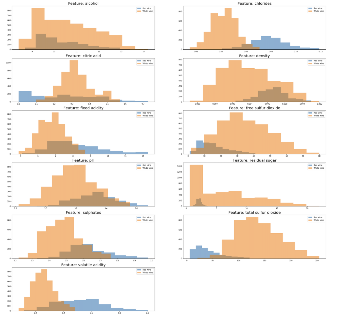
어떤 설명변수가 와인의 종류를 결정 짓는지 그래프를 히스토그램으로 시각화하여 살펴본 결과
레드 와인과 화이트 와인을 각각 histogram으로 나타냄
두 그래프가 겹치는 구간이 적다는 것은 해당 설명 변수에 의해 와인 종류를 분류할 가능성이 크다는 의미임
9. 데이터 스케일링
설명변수마다 데이터 범위 차이가 크기 때문에 표준 스케일러인 StandardScaler로 데이터 스케일링 수행
표준 스케일러는 평균을 0으로 분산을 1로 스케일링
목표 변수는 스케일링할 필요가 없기 때문에 설명 변수만 스케일링 진행
# 표준 스케일러(평균 0, 분산 1)
scaler = StandardScaler()
# 설명변수 및 목표변수 분리
x = df[df.columns.difference(['target'])]
y = df['target']
# 설명변수 데이터 스케일링
x_scaled = scaler.fit_transform(x)
10. 학습/테스트 데이터 분리
# 학습, 테스트 데이터셋 7:3 비율로 분리
x_train, x_test, y_train, y_test = train_test_split(x_scaled, y,
                                                    test_size = 0.3, random_state = 42)
 # 훈련 데이터 내 와인별 비율
y_train.value_counts(normalize=True)

# 테스트 데이터 내 와인별 비율
y_test.value_counts(normalize=True)
모델링
하이퍼 파라미터 튜닝없이 모델 학습 및 성능 평가
파라미터로 알고리즘 종류와 설명변수 x, 목표 변수 y의 훈련/테스트 데이터를 전달 받음
def modeling_uncustomized (algorithm, x_train, y_train, x_test, y_test):
    # 하이퍼파라미터 조정 없이 모델 학습
    model = algorithm(random_state=42)
    model.fit(x_train, y_train)
    # Train Data 설명력
    train_score_before = model.score(x_train, y_train).round(3)
    print(f"학습 데이터셋 정확도: {train_score_before}")
    # Test Data 설명력
    test_score_before = model.score(x_test, y_test).round(3)
    print(f"테스트 데이터셋 정확도: {test_score_before}")
    return train_score_before, test_score_before
학습
하이퍼 파라미터 튜닝 없이 기본 모델 학습
train_acc_before, test_acc_before = modeling_uncustomized(algorithm,
                                                          x_train,
                                                          y_train,
                                                          x_test,
                                                          y_test)
학습 데이터 기반 분류 모델 정확도가 100인 경우 과대 적합 발생
하이퍼 파라미터 튜닝을 통해 과대 적합 방지 필요
최적화
1. 하이퍼 파라미터 모델 성능 시각화
하이퍼 파라미터 튜닝에 따라 모델 성능이 어떻게 달라지는지 추이 확인
하이퍼파라미터 값을 x축
y축은 학습 및 테스트 데이터 기반 모델 정확도 측정
def optimi_visualization(algorithm_name, x_values, train_score, test_score, xlabel, filename):
    # 하이퍼파라미터 조정에 따른 학습 데이터셋 기반 모델 성능 추이 시각화
    plt.plot(x_values, train_score, linestyle = '-', label = 'train score')
    # 하이퍼파라미터 조정에 따른 테스트 데이터셋 기반 모델 성능 추이 시각화
    plt.plot(x_values, test_score, linestyle = '--', label = 'test score')
    plt.ylabel('Accuracy(%)') # y축 라벨
    plt.xlabel(xlabel) # x축 라벨
    plt.legend() # 범례표시
    plt.savefig('../figure/' + algorithm_name + '_' + filename + '.png') # 시각화한 그래프는 로컬에 저장
2. 트리 모델 개수 선택
트리 개수를 5개씩 최대 트리 개수까지 늘려가면서 모델 성능 평가
모델 성능은 앞서 언급한 시각화 함수에 전달하여 성능 변화 추이 시각화
def optimi_estimator(algorithm, algorithm_name, x_train, y_train, x_test, y_test, n_estimator_min, n_estimator_max):
    train_score = []; test_score =[]
    para_n_tree = [n_tree*5 for n_tree in range(n_estimator_min, n_estimator_max)]

    for v_n_estimators in para_n_tree:
        model = algorithm(n_estimators = v_n_estimators, random_state=42)
        model.fit(x_train, y_train)
        train_score.append(model.score(x_train, y_train))
        test_score.append(model.score(x_test, y_test))

    # 트리 개수에 따른 모델 성능 저장
    df_score_n = pd.DataFrame({'n_estimators': para_n_tree, 'TrainScore': train_score, 'TestScore': test_score})
    # 트리 개수에 따른 모델 성능 추이 시각화 함수 호출
    optimi_visualization(algorithm_name, para_n_tree, train_score, test_score, "The number of estimator", "n_estimator")
    print(round(df_score_n, 4))
n_estimator_min = 1
n_estimator_max = 31
optimi_estimator(algorithm, algorithm_name,
                 x_train, y_train, x_test, y_test,
                 n_estimator_min, n_estimator_max)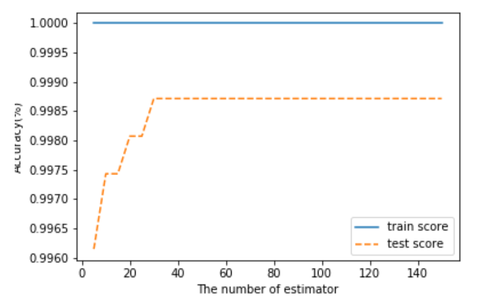
학습 데이터 기반 모델 정확도가 100으로 여전히 과적합 발생 중
트리 개수는 많을 수록 과적합 방지에 유리함
학습 데이터 기반 모델 정확도와 테스트 데이터 기반 모델 정확도의 차이가 적을수록 좋음
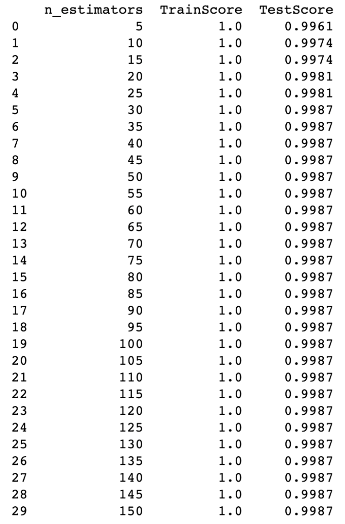
트리 개수를 30으로 선정
트리 개수가 30일 때 테스트 데이터 기반 모델 정확도가 가장 높음
n_estimator = 30
3. 모델이 학습할 트리별 최대 깊이 결정
최대 깊이를 지정한 최솟값부터 1씩 늘려가면서 최댓값까지 모델의 성능 평가
def optimi_maxdepth (algorithm, algorithm_name, x_train, y_train, x_test, y_test, depth_min, depth_max, n_estimator):
    train_score = []; test_score = []
    para_depth = [depth for depth in range(depth_min, depth_max)]

    for v_max_depth in para_depth:
        # 의사결정나무 모델의 경우 트리 개수를 따로 설정하지 않기 때문에 RFC, GBC와 분리하여 모델링
        if algorithm == DTC:
            model = algorithm(max_depth = v_max_depth,
                              random_state=42)
        else:
            model = algorithm(max_depth = v_max_depth,
                              n_estimators = n_estimator,
                              random_state=42)

        model.fit(x_train, y_train)
        train_score.append(model.score(x_train, y_train))
        test_score.append(model.score(x_test, y_test))

    # 최대 깊이에 따른 모델 성능 저장
    df_score_n = pd.DataFrame({'depth': para_depth, 'TrainScore': train_score, 'TestScore': test_score})
    # 최대 깊이에 따른 모델 성능 추이 시각화 함수 호출
    optimi_visualization(algorithm_name, para_depth, train_score, test_score, "The number of depth", "n_depth")
    print(round(df_score_n, 4))
depth_min = 1
depth_max = 21
optimi_maxdepth(algorithm, algorithm_name,
                x_train, y_train, x_test, y_test,
                depth_min, depth_max, n_estimator)
최대 깊이에 대한 학습 및 테스트 데이터의 모델 성능 확인
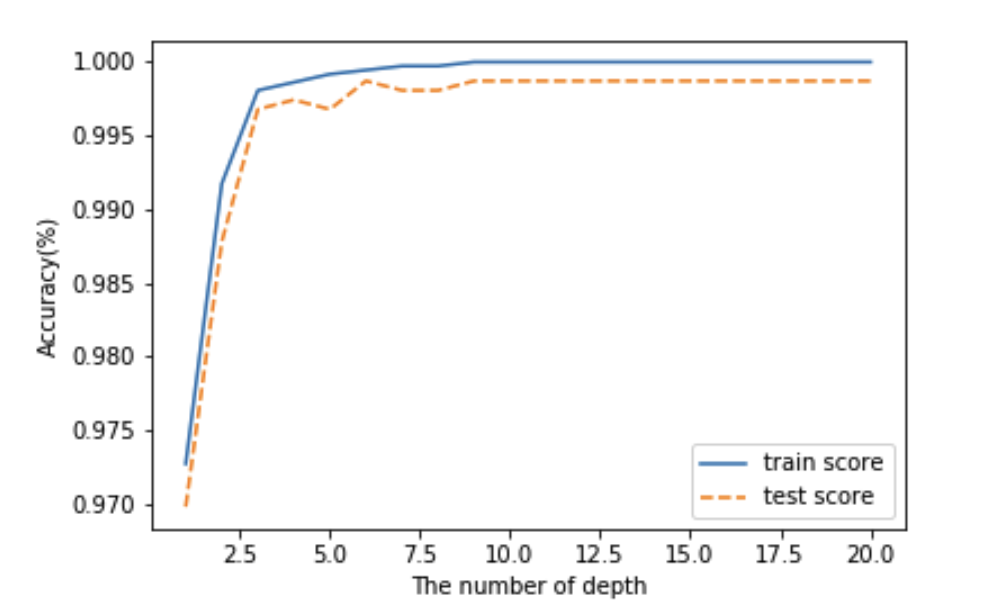
최대 깊이는 적을 수록 유리함
그렇기 때문에 최대 깊이가 적고 훈련 데이터 기반 모델 성능이랑 테스트 데이터 기반 모델 성능 간의 차이가 적은 값을 선정하는 것이 유리함
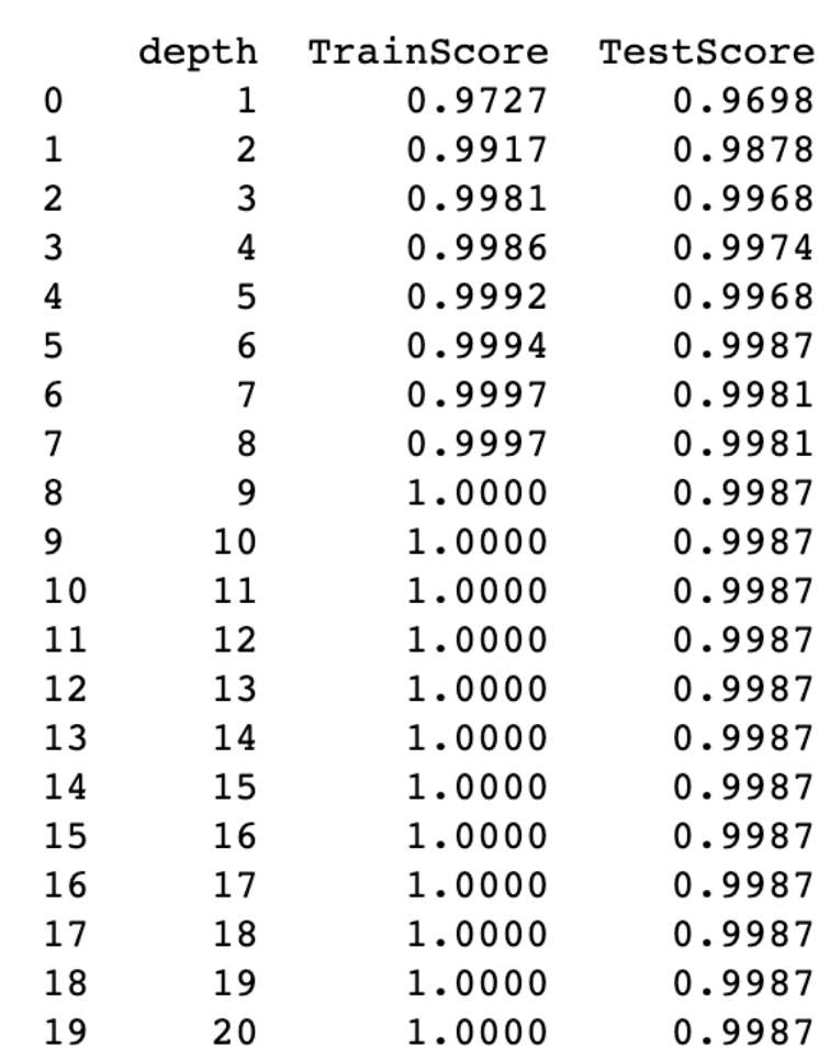
트리 깊이가 최대한 적고 테스트 기반 모델 정확도가 증가하다가 감소하는 구간인 최대 깊이 6으로 트리 깊이 지정
트리 깊이는 6
n_depth = 6
4. 분리 노드의 최소 자료 수 선택
모델에 대한 최적화 함수의 정의는 생략
분리 노드의 최소 자료 수가 많을수록 과적합 방지에 유리함
분리 노드의 최소 자료 수는 66으로 선정
n_split = 66
5. 잎사귀 노드의 최소 자료 수 선택
모델에 대한 최적화 함수의 정의는 생략
잎사귀 노드의 최소 자료 수는 많을수록 과적합 방지에 유리함
잎사귀 노드의 최소 자료 수는 20으로 선정
n_leaf = 20
6. 최종 학습
앞에서 구한 최적의 하이퍼 파라미터를 기반으로 최종 모델 학습
pickle 모듈을 통해 학습한 모델 저장
모델 성능 평가를 위해 accuracy, precision, recall, confusion matrix, f1 score, recall 활용
마지막으로 변수별 중요도 산출 및 시각화
def model_final(algorithm, algorithm_name, feature_name, x_train, y_train, x_test, y_test, n_estimator, n_depth, n_split, n_leaf):
    # 의사결정나무 모델의 경우 트리 개수를 따로 설정하지 않기 때문에 RFC, GBC와 분리하여 모델링
    if algorithm == DTC:
        model = algorithm(random_state=42,
                          min_samples_leaf = n_leaf,
                          min_samples_split = n_split,
                          max_depth = n_depth)
    else:
        model = algorithm(random_state = 42,
                          n_estimators = n_estimator,
                          min_samples_leaf = n_leaf,
                          min_samples_split = n_split,
                          max_depth = n_depth)
    # 모델 학습
    model.fit(x_train, y_train)
    # 모델 저장
    model_path = '../model/'
    model_filename = 'wine_classification_' + algorithm_name + '.pkl'
    with open(model_path + model_filename, 'wb') as f:
        pickle.dump(model, f)
    print(f"최종 모델 저장 완료! 파일 경로: {model_path + model_filename}\n")

    # 최종 모델의 성능 평가
    train_acc = model.score(x_train, y_train)
    test_acc = model.score(x_test, y_test)
    y_pred = model.predict(x_test)
    print(f"Accuracy: {accuracy_score(y_test, y_pred):.3f}") # 정확도
    print(f"Precision: {precision_score(y_test, y_pred):.3f}") # 정밀도
    print(f"Recall: {recall_score(y_test, y_pred):.3f}") # 재현율
    print(f"F1-score: {f1_score(y_test, y_pred):.3f}") # F1 스코어

    # 혼동행렬 시각화
    plt.figure(figsize =(30, 30))
    plot_confusion_matrix(model,
                         x_test, y_test,
                         include_values = True,
                         display_labels = ['Red', 'White'], # 목표변수 이름
                         cmap = 'Pastel1') # 컬러맵
    plt.savefig('../figure/' + algorithm_name + '_confusion_matrix.png') # 혼동행렬 자료 저장
    plt.show()

    # 변수 중요도 산출
    dt_importance = pd.DataFrame()
    dt_importance['Feature'] = feature_name # 설명변수 이름
    dt_importance['Importance'] = model.feature_importances_ # 설명변수 중요도 산출

    # 변수 중요도 내림차순 정렬
    dt_importance.sort_values("Importance", ascending = False, inplace = True)
    print(dt_importance.round(3))
    # 변수 중요도 오름차순 정렬
    dt_importance.sort_values("Importance", ascending = True, inplace = True)
    # 변수 중요도 시각화
    coordinates = range(len(dt_importance)) # 설명변수 개수만큼 bar 시각화
    plt.barh(y = coordinates, width = dt_importance["Importance"])
    plt.yticks(coordinates, dt_importance["Feature"]) # y축 눈금별 설명변수 이름 기입
    plt.xlabel("Feature Importance") # x축 이름
    plt.ylabel("Features") # y축 이름
    plt.savefig('../figure/' + algorithm_name + '_feature_importance.png') # 변수 중요도 그래프 저장
from sklearn.ensemble import RandomForestClassifier as RFC # 랜덤포레스트 분류 알고리즘
from sklearn.tree import DecisionTreeClassifier as DTC
# 랜덤포레스트 분류 알고리즘
algorithm = RFC
algorithm_name = 'rfc'
model_final(algorithm, algorithm_name, feature_name,
            x_train, y_train, x_test, y_test,
            n_estimator, n_depth, n_split, n_leaf)
'인공지능 > machine learning' 카테고리의 다른 글
| [ML] 부스트코스 Data Scientist Projects 2024 1주차 (0) | 2024.01.17 |
|---|---|
| [DL] 모두를 위한 딥러닝 노트 정리 (2/2) (0) | 2023.12.08 |
| 분류(Classification) vs 회귀(Regression) 문제 구분하기 (+평가 지표 정리 Confusion Matrix, Precision, Recall, f1-score, ROC, AUC, MAE, MSE, RMSE, ...) (1) | 2023.11.16 |
| [ml] 머신러닝 예측 regression 문제 뽀개기 (0) | 2023.11.15 |
| [ml] 머신러닝 예측/분류 문제를 풀기 위한 Tips (0) | 2023.11.15 |


